
Half-sibling Regression
Half-sibling model
Half-sibling regression is an approach to de-noise data that follows the following model, with true signal $Q$ and measurement $Y$ which has noise added due to $N$. Crucially there are other variables we have measured which are affected by the same noise but are independent of the true signal $Q$. We call these variables $X_1, X_2$ half-siblings of $Y$.
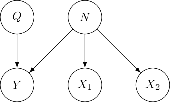
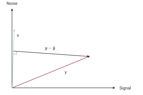
The idea is to regress $Y$ on its half-siblings $X_1, X_2, \dots X_k$. Since the half-siblings are independent of the true signal, anything shared by $Y$ and any half-sibling must correspond to noise from $N$. This is shown in this (slightly terrible) diagram, where I have written $y$ as a vector which is a combination of true signal and noise. In terms of the true signal (of $y$) and noise, $x$ corresponds almost entirely to noise. Of course, $x$ should really be shown as a combination of noise and its true signal, which we could show using a 3rd axis.
When we regress $y$ on its half-sibling $x$, we recover $\hat{y}$ which is in the same direction as $x$. The residuals $y-\hat{y}$ are then almost in the same direction as the signal i.e. we have recovered the part of $y$ that is due to signal.
Example application - searching for exoplanets
I came across this method in a lecture series by Jonas Peters on causality, where he used it as an example of how thinking about the causal structure of data can help to suggest statistical methods for their analysis. In the course Peters gives the example from (Schölkopf et al. 2016) of measurements of light intensity of various points in the sky as measured by the Kepler space observatory. The aim is to detect troughs of light intensity, as if there are regular troughs this might correspond to an exoplanet orbiting a star.
My example - noisy measurements of weight
To explore this idea I decided to simulate some data from the following model:
The weights of 20 individuals are measured every week for 20 weeks. We want to understand how the weights change over the study, for example we might be interested in understanding the impact of diet on weight. However, let’s suppose the weighing scales we use are calibrated each week in an inconsistent fashion, so that we cannot directly compare a measurement from week 1 to week 2. If we simply considered the weight of each individual in isolation we would have no way to remove the noise. However, by using half-sibling regression we can remove much of the noise.
set.seed(13)
n_inds <- 10
n_weeks <- 20
between_individual_sd <- 20
within_invividual_sd <- 10
measurement_noise_sd <- 20

# Simulate baseline weights for each individual - weekly fluctuations will be relative to this baseline
baseline_weights <- rnorm(n_inds, mean=80, sd=between_individual_sd)
baseline_weights[1:5]
## [1] 91.08654 74.39456 115.50327 83.74640 102.85052# Add weekly fluctuations for each individual
weekly_weights_true <- matrix(rnorm(n_inds*n_weeks,
mean=rep(baseline_weights, n_weeks),
sd=within_invividual_sd),
ncol=n_inds,
byrow=TRUE)
measurement_noise <- rnorm(n_weeks, mean=0, sd=measurement_noise_sd)
weekly_weights_measured <- data.frame(weekly_weights_true + matrix(rep(measurement_noise, n_inds), ncol=n_inds))
weekly_weights_measured$week <- as.factor(1:n_weeks)
weekly_weights_measured[1:8, 1:5]## X1 X2 X3 X4 X5
## 1 43.86698 42.72965 65.60981 28.90251 62.16835
## 2 97.50977 96.55400 122.87509 77.09010 112.85017
## 3 73.65365 65.52176 94.31757 61.13051 82.76748
## 4 101.34081 99.54576 130.41908 109.14206 107.41489
## 5 60.20263 48.33461 78.39788 44.66929 71.57894
## 6 104.09525 103.00173 139.64965 100.48163 138.60564
## 7 58.39564 51.95721 88.51341 42.84679 82.09921
## 8 95.37199 82.41576 108.60579 68.82372 121.78172In this plot of the measurements throughout the year we see that there is a similar pattern for each individual, caused by the shared measurement noise. This structure is what we will exploit to recover the true signal.
# Transform the data so that each row corresponds to a single measurement,
#   with the 'week' column still giving the week of the measurement and
#   the 'individual' column giving the ID of the individual
ggplot(pivot_longer(weekly_weights_measured,
                    cols=-week,
                    names_to="individual",
                    values_to="measured_weight"),
       aes(x=week, y=measured_weight, colour=individual, group=individual)) +
  geom_line()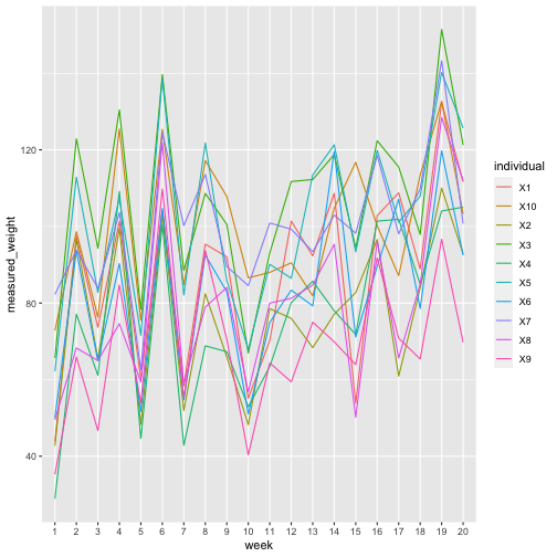
We now fit the half-sibling regression model, regressing one of the variables $X_1$ on its half-siblings. In R we specify this with the formula “X1 ~ . -week” meaning “regress X1 on all the remaining variables except for ‘week’”.
model <- lm(X1 ~ . - week, data=weekly_weights_measured)
print(model)
##
## Call:
## lm(formula = X1 ~ . - week, data = weekly_weights_measured)
##
## Coefficients:
## (Intercept) X2 X3 X4 X5 X6 X7 X8
## -2.11320 -0.20322 0.48235 0.27218 -0.10304 0.48817 -0.07079 0.30369
## X9 X10
## -0.12539 -0.05352We can now construct our predictions using the residuals of the regression model.
# Construct a data frame with useful columns for each week (sample) for this individual (variable X1)
x1_measurements <- data.frame(week=weekly_weights_measured$week,
                      individual="X1",
                      x1_measured=weekly_weights_measured$X1,
                      x1_true=weekly_weights_true[, 1],
                      noise=measurement_noise,
                      x1_pred=model$residuals + mean(weekly_weights_measured$X1),
                      x1_residuals=model$residuals)

# Sum of squared error of measurement compared to true value
true_fluctuations <- x1_measurements$x1_true - baseline_weights[1]
measured_fluctuations <- x1_measurements$x1_measured - baseline_weights[1]
print(sum((true_fluctuations - measured_fluctuations)**2))
## [1] 6860.143# Sum of squared error of predicted compared to true value
print(sum((true_fluctuations - model$residuals)**2))## [1] 2041.594So we have achieved significant noise reduction, though we are still not perfectly recovering the signal even in this case where the noise has mean 0. Now we can plot the true signal, noisy signal and our predictions using half-sibling regression. In each case the black line shows the baseline value as a reference. Since the noise had mean 0 our predictions fluctuate about this line.
# Pivot so we have a row for each weight value, with a new column 'name' giving the type of measurement (true, predicted, measured)
ggplot(pivot_longer(x1_measurements, cols=x1_measured:x1_pred),
       aes(x=week, group=name)) +
  geom_line(aes(y=value, colour=name)) +
  #geom_smooth(method='lm', mapping=aes(y=value), formula=y~x) +
  geom_hline(yintercept=baseline_weights[1], colour='grey') +
  facet_wrap(~name, ncol=1)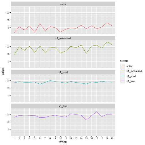
Note for example in this graph that the noise variable has a large increase in week 6, but the true value has a decrease in week 6. The measured value obviously shares the increase from the noise variable, but we have managed to predict a decrease, matching the pattern of the true signal.
Further questions
How can we quantify noise reduction?
Does this work when the noise doesn’t have zero mean? Or when the signal is increasing? E.g. if the weight is increasing over time, will we recover this upwards trend? What if the noise is decreasing to balance the increase? I think a key thing that needs to be achieved is independence of noise and signal. At one point I tried increasing the signal (for only one variable) at the same rate as decreasing the noise, but this effectively means that the two are dependent (in this case if this decrease/increase is strong compared to the other changes occurring, the two will be inversely correlated and thus dependent).
Note that this is only valid if all individuals are truly independent. Perhaps if they weren’t all independent (e.g. if they were all following the same diet/exercise plan) we would have to regress only on the genuine half-siblings e.g. regress a control sample on treatment samples and regress a treatment sample only on control samples.
Sources
I used this guide to draw the DAG using latex.
Bernhard Schölkopf et al., ‘Modeling Confounding by Half-Sibling Regression’, Proceedings of the National Academy of Sciences 113, no. 27 (5 July 2016): 7391–98, https://doi.org/10.1073/pnas.1511656113.